One of the advantages of Python is the large ecosystem of libraries for handling numerical problems. There are good reasons to use these from .Net/CLR/C# applications with their high reliability, and excellent tooling and large enterprise code bases. Fortunately thare are several ways of doing this.
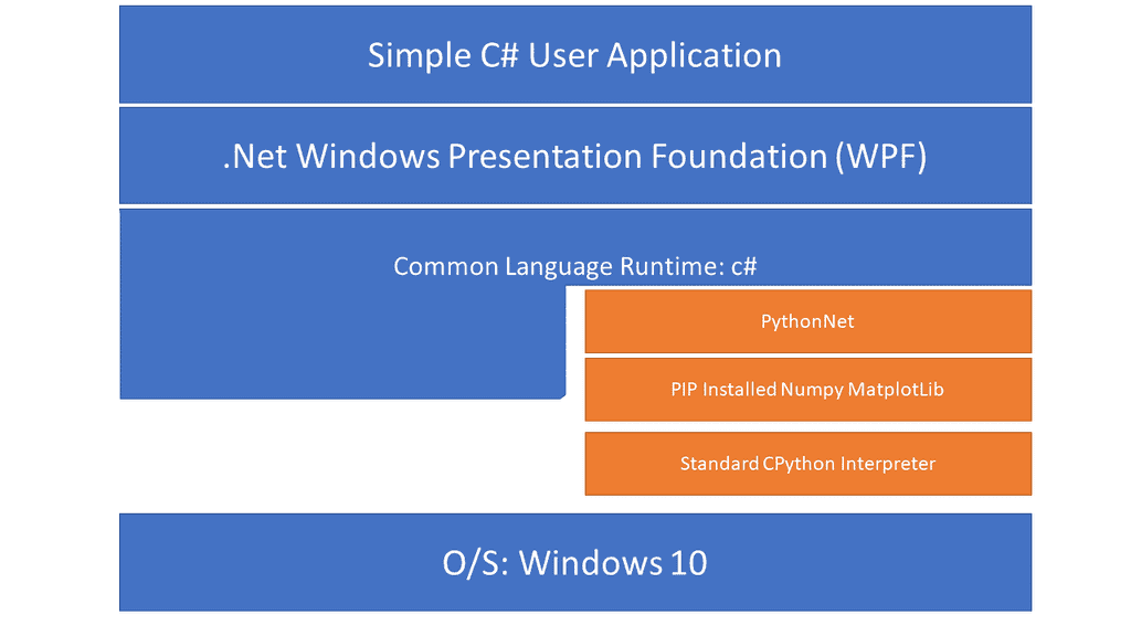
One of the ways of implementing this is shown below:

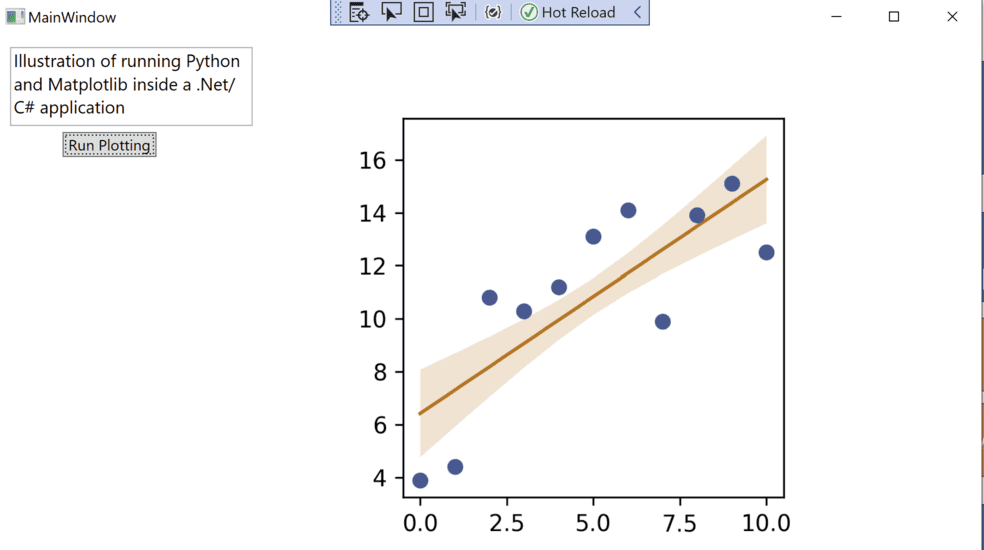
It consists of using the PythonNet library to load the CPython interpreter in-process to the .Net application and allow access to all of the Python libraries. As shown above, this can be used, for example, to draw technical figures and graphs using matplotlib many capabilities.
The above example is our own implementation. The Matplotlib.net uses similar approach but unfortunately has not progressed for last few years. There is also MatplotlibCS which implements the communication between Python and NET CLR via HTTP network requests. In MatplotlibCS the plot to be made is represented by as JSON object. In an in-process implementation like ours the plot can be imperatively built using standard function calls.
Some of the features of our approach:
- Python interpreter, Matplotlib and necessary python libraries bundled together in the .Net assembly together with the wrapping
- Installable with NuGet
- Resource-efficient and reliable due to in-process union of the Python part and the the C# parts.
If you need help with these integrations contactact us at: info@quantfns.com . For more information see our dedicated pages at www.quantfns.com/pyinnet/.

Here is the source code extract -- please contact us for more details!
private void Button_Click(object sender, RoutedEventArgs e)
{
    int dpi = 300;
	BitmapSource bitmap;

    PythonEngine.Initialize();
    using (Py.GIL())
    {
        dynamic npi = Py.Import("numpy");

        int N = 21;
        var x = np.linspace(0, 10, 11);
        var y = np.array(new double[] {  3.9, 4.4, 10.8, 10.3, 11.2, 13.1, 14.1, 9.9, 13.9, 15.1, 12.5 });
        var fitr = npi.polyfit(x.PyObject, y.PyObject, deg: 1);
		double a = fitr[0];
		double b = fitr[1];

        var y_est = a * x + b;

        var y_err = x.std() * np.sqrt( np.power((x - x.mean()), np.array(2)) / np.sum(np.power((x - x.mean()) , np.array(2))) +1.0 / N );

        (var pyfig,  var ax) = pyplot.subplots(figsize: new List<double> { 3, 3 }, dpi: dpi);
        ax.plot(x, y_est, '-');
        ax.fill_between(x, (y_est - y_err),
	                    (y_est + y_err),
                        alpha: 0.2);
        ax.plot(x, y, 'o',
		color : "tab:brown");
		bitmap = pyfig.bitmap();
    }

    // Create an image element;
    img1.Source = bitmap;

}
